AH EPISODES

There are multiple ways to access the AH Episode data available in the IS-EPOS.The User may click on the "AH Episodes" tab from the portal menu on the upper left corner of the screen (Field 1, Figure 1). In such way the available episodes are displayed on the screen along with options for selecting/filtering. "Advanced data search" (field 2, Figure 1) will be described later on. The User is provided the possibility for selecting among AH Episodes according to technology/production process they are connected with. This can be done by ticking the small boxes shown in field 3 of Figure 1. Ticking "All" box, will exclude no Episode from the list displayed (field 4, figure 4). The User can now click on one of the Episodes (e.g. Bobrek Mine, or Czorsztyn) from this list to get access to the corresponding data.

Figure 1.

For each one of the AH Episodes from the list, some short information concerning the technology and the region associated with the Episode is provided. In addition, a world map is shown in the lower part of the screen with the location of the selected episodes indicated (Figure 2). Zooming, map/satellite view, drawing of national borders and full screen mode are options provided for the map handling.

Figure 2.

Figures 3 and 4 show an example of a page with data from Bobrek Mine Episode. The structure and interface is identical in all cases. Some informative fields are displayed in the upper part of the screen such as the Episode State, Industrial process and Region, together with a short Description of the Episode (Figure 3). Some figures connected with the selected Episode are also displayed, providing additional information. Episode Data is found just below the Description and are categorized into 3 groups with different data types (Field 1, Figure 4): Seismic data, Technological data and Geological data

Figure 3.

Seismic Data includes mainly seismity catalogs, seismic network information and waveforms corresponding to seismic events as they were recorded by the stations. Geological data include mainly velocity models from the site of the Episode and maps with local faulting systems. On the other hand, Technological data contains a group of data files which is directly connected with the technological-production processes that induce the anthropogenic seismicity (see the example from Bobrek Mine, Figure 4).

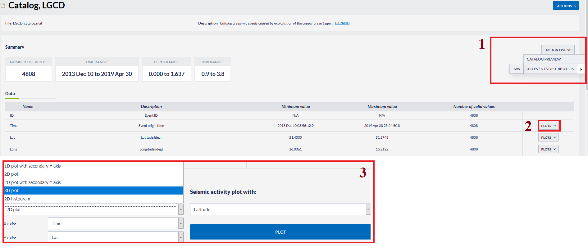
Figure 4.

There are additional fields shown in Figure 4: Field 2, "All data related to this episode", gives access to the "Advanced data search", which will be described later on. "Available visualizations" (field 3, Figure 4) provides to the User the ability to perform integrated Episode data visualization and various other visualizations, regarding the selected Episode. Finally clicking on field 4, "See more information in Document Repository", leads the User to the document repository engine, to seek for references and further details concerning the Episode, data, methods etc.

All of the aforementioned data sets can be selected and then added to workspace and be used in the available services. For some of these data sets, visualization is also shown, as map view (e.g. Seismic Network, mining area, reservoir shoreline) or graph charts (e.g. Velocity model, mining front advance, injection rate). The map view - like data can be combined and demonstrated in a single map by selecting the "integrated Episode data visualization" from the "Available Visualizations" tab. Seismic events (red circles), network of seismic stations (green triangles) and various episode-related data can be shown/hidden by setting/deleting a tick in the small boxes shown in the upper part of figure 5.

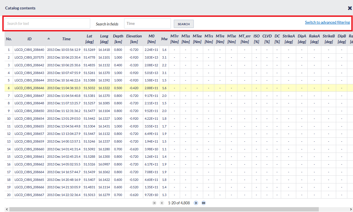
Figure 5.

Additional options are available for some specific kinds of data (Catalog and Water Level/ Wellhead pressure with seismic activity, e-D visualization and Integrated GIS data), therefore, these will be now described in detail.

Catalog Options (All episodes)

Seismic catalog contains various important information as demonstrated in Figure 6 and Figure 7. The User may upload the catalog data in the workspace by selecting "Actions" (field 1, Figure 6) and then "Add to workspace". Below this field, a short summary of the catalog is provided, containing the number of events, time range, depth range and magnitude range. Below the summary, there are some action tabs (fields 2-6, Figure 6). The attributes of the catalog are displayed below these tabs, and they comprise the Name of the attribute, a brief description, the minimum and maximum values and the number of valid values. The action tabs are the following:

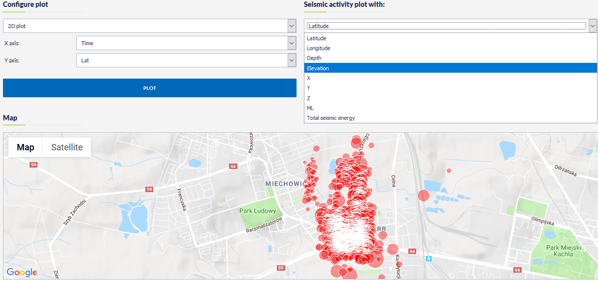
Figure 6.

Seismic Activity Step plot (field 2, Figure 6): Seismic activity plotted against time (Figure p1). Zooming in/out and linear/logarithmic y-axis are available.

Figure p1.

3D events distribution (field 3, Figure 6): 3D spatial distribution of the events foci (longitude,latitude,depth), as circles with size proportional to the event magnitude (Figure p2). Rotation of the plot is possible after clicking and dragging the cursor through the plot area. The focal coordinates of each event are depicted when the cursor is pointing on a circle.

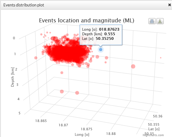
Figure p2.

Benioff plot (field 4, Figure 6): A Benioff plot (square root of energy against time) can be created for those catalogs which include information on seismic energy released by the events (Figure p3). Zooming in/out and linear/logarithmic y-axis are available.

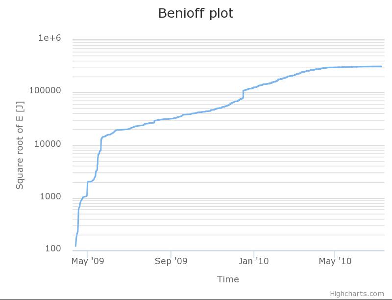
Figure p3.

Show catalog (field 5, Figure 6): Detailed information on the attributes of every event in the seismic catalog is demonstrated (Figure p4). These data appear as pop-up windows and are shown in pages, each one containing 20 rows. The User can proceed to the following of previous pages by clicking the left-right arrows shown in the lower left part of Figure p4.

Figure p4.

Events in local coordinates (field 6, Figure 6): 2-D plot of the epicentral coordinates of the seismic events (Figure p5) in local (cartesian) coordinate system (when these are available). Zooming in/out option is available.

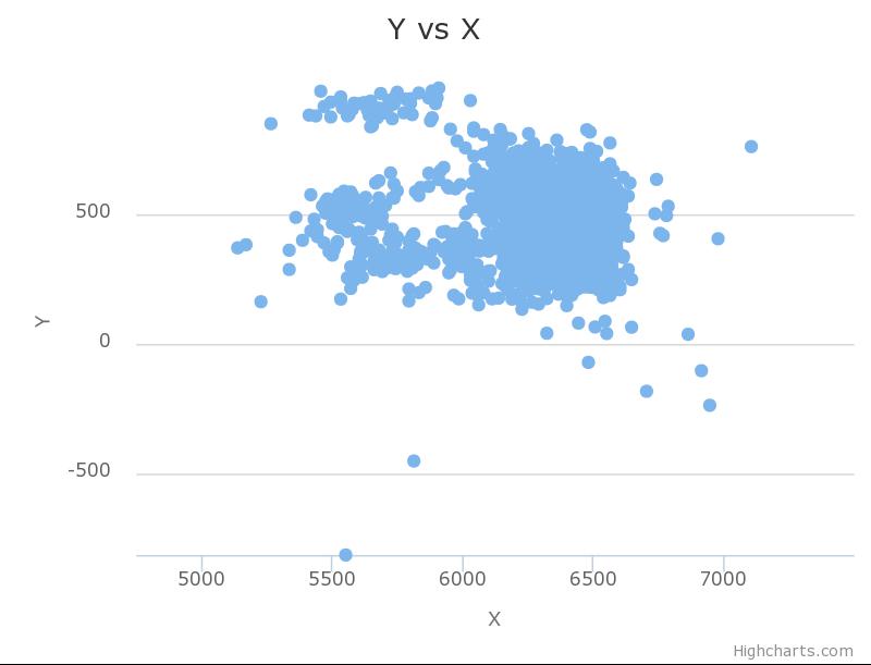
Figure p5.

Additional plotting options are available be clicking on the gear icon shown in field 7 of Figure 6 (right hand side). These options include histograms (interval, cumulative and reversed cumulative histograms) and 1-D plots. Zooming in/out and linear/logarithmic y-axis are available. Moreover, in histograms the bar step can be modified and in 1-D plots the chart type can be switched among column, scatter, spline and line.

Even more visualization options are available in the lower part of the screen, as shown in Figure 7. The epicenters of the seismic events are demonstrated on a google map, which provides zooming, map/satellite view, drawing of national borders and full screen mode are options. The events serial numbers, their origin time and the magnitudes, are shown in the screen after the User clicks on one of the events depicted by the red circles. A variety of plots are available as shown in field 1, Figure 7. The User can chose one of the following plot types, defining the attribute to be shown at the X, Y and Z axis:

1-D plot with secondary Y-axis (zooming in/out and linear/logarithmic x-axis and y-axis are available)
2-D plot (zooming in/out and linear/logarithmic x-axis and y-axis are available)
2-D plot with secondary Y-axis (zooming in/out and linear/logarithmic x-axis and y-axis are available)
3-D plot (rotation of the plot is possible after clicking and dragging the cursor through the plot area)
2-D Histogram, as shown in Figure 8 (rotation of the plot is possible after clicking and dragging the cursor through the plot area).

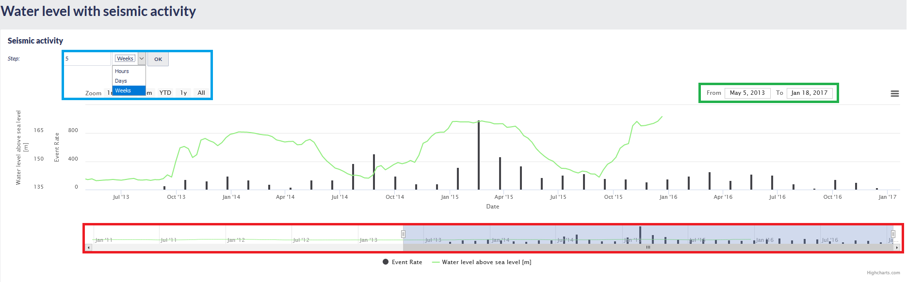
Figure 7.

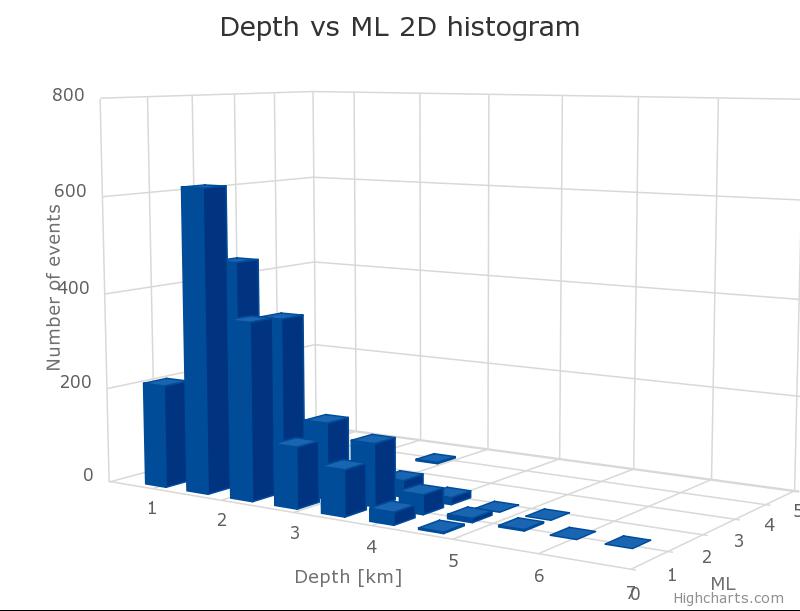
Figure 8.

Finally, seismic activity can be plotted together with any other parameter in Field 2 of Figure 7. An example of seismic activity plotted with latitude is shown in Figure 9. The time step can be set by the User. The time unit can be chosen as well among hour, day and week. Zooming in/out and linear/logarithmic y-axis are available for this plot.

Figure 9.

Water Level/ Wellhead pressure with Seismic Activity (Czorsztyn, Gross Schoenebeck and Song Tranh)

In this service the technological activity (either reservoir water level or wellhead pressure) is plotted in the same diagram with the histogram of the seismic activity. There are options for both parameters as shown in Figure 10. The step and time unit (hours, days or weeks) of the seismic activity can be selected for the histograms of seismicity. On the other hand the plot mode of the water level can be adjusted as well, as simple, cumulative, gradient and average (Figure 10).

The zooming (in the X-axis) can be performed in two ways: First by selecting a predefined time unit, shown after "Zoom" field, among 1 month, 3 months, 6 months, YTD???, 1 year and all (i.e. the entire period). The second is to interactively zoom in/out the X-axis on the lower frame (shown in the red box in Figure 10). The User has just to click on the small rectangles in the left and right of the shaded panel and drag them to either direction in order to select the time period he/she wishes. The selected period can be shifted towards left/right by either dragging the cursor after clicking into the shaded part, or by using the small arrows at the left and right bottom corner of the lower figure. In any case the starting and ending date of the chosen period is noted in the screen (green box in Figure 10).

Figure 10.

3-D Visualizations (Gross Schoenebeck)

... to be completed

The objects manager can be user at any time in order to hide/show selected objects on the screen such as the injection wells, the seismic events, the stations of the seismic network, the surface map and the map scale.

Figure 11.

Integrated GIS data (Bobrek)

This service allows User to integrate GIS data into an interactive base map plot.

Figure 12.