User Guide Fracture Network Models - Mechanical Stresses

Fracture Network Models - Mechanical Stresses

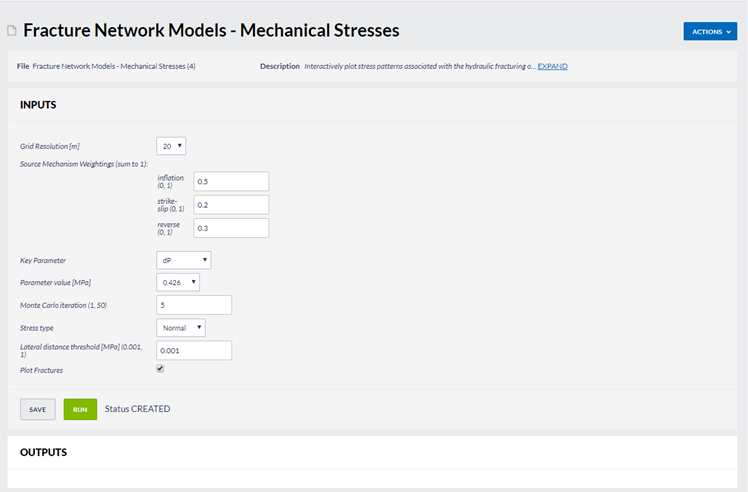
Figure 1. The options available for the service

About the Service

This service interactively plots stress patterns associated with the hydraulic fracturing of a shale gas well.

The data is based on the physical and geological conditions at the Preese Hall Episode site.

The application allows you to produce Coulomb, Normal or Shear stress maps for a specific source mechanism weighting and key parameter.

Also calculated is the lateral respect distance, that is the minimum distance that fracking should

occur from a pre-existing critical fault in order not to reactivate it.

The modelling which is used to create the plot is explained in the reference document - Westwood, R. F., Toon, S. M. & Cassidy, N. J., 2017. A sensitivity analysis of the effect of pumping parameters on hydraulic fracture networks and local stresses during Shale Gas operations.

License Terms

This work is licensed under a Creative Commons Attribution-ShareAlike 4.0 International License.

For full details of the license see https://creativecommons.org/licenses/by-sa/4.0/legalcode.

Inputs

Grid Resolution: This is the resolution of the grid used for the stress map. Options are:

-      50 m – this produces a stress map 4 km x 4 km with 50 m spacing; or

-      20 m – this produces a stress map 1 km x 1 km with 20 m spacing.

Source Mechanism Weightings: Here you can specify the source mechanism used to generate the

fractures as a ratio between inflation, reverse and strike-slip. Values should be between 0 and 1 and must total 1.

Key Parameter: The stress calculation is based on this parameter. Options are:

-      dP – This is the pressure difference between pore pressure and normal pressure on the

fractures at injection.

-      FlowRate - Fluid is injected into the well at this rate.

-      PumpTime - This is the length of time that the fluid is pumped into the well.

Parameter Value: The value of the key parameter you selected in MPa for dP, m3

/s for flow rate and minutes for pump time.

Monte Carlo iteration: The simulations were run for 50 Monte Carlo iterations, generating a new

discrete natural fracture network each time, so the results are each slightly different. Enter the

iteration you wish to visualise here.

Stress type: Select whether you wish to visualise Normal, Shear or Coulomb stress.

Lateral distance threshold: Enter the threshold value in MPa to use to define the stress required to

reactive a critical fault. Values typically range from 0.001-0.1 MPa.

“Freed (2005) uses aftershock studies to define triggering at 0.1 MPa to 0.3 MPa or less. Kilb

et al. (2002) state that the optimal triggering threshold is 0.1 MPa, but find correlations with

seismicity rate change for value between 0.001 MPa and 0.5 MPa. The results of Shapiro et

al. (2006) also indicate that triggering occurs as low as 0.001 - 0.1 MPa.” Westwood et al.

(under review)

Plot Fractures: Tick this box if you wish to plot the fractures.

Outputs

Two outputs are generated: a jpg of the stress map and a text file containing additional information.

JPG Stressmap: The algorithms described by Okada [28] are used to calculate failure on optimally orientated strikeslip faults. The calculation is performed at each point of a discretized cube. A 2D stress map is obtained by calculating the maximum and minimum stresses over depth, resulting in a map like the one provided in Figure 2. The maximum and minimum stresses are indicated by the black and grey lines respectively at 0.00001 MPa (50 m) and 0.000001 MPa (20 m) intervals.

Text file The text file (see Figure 3 for an example) contains additional information about the calculation inputs.

The first section of the text file states the key parameter and parameter value used for the

calculation and the Monte Carlo iteration.

The second and third blocks contain the geological parameters and regional stresses, respectively,

used in the calculation.

The final block states the threshold value used for the lateral respect distance and the mean,

median, maximum and minimum lateral respect distances over all 50 Monte Carlo iterations.

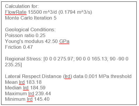
Figure 2. Example text file output

MAT file: The stress plot data saved in a MAT file

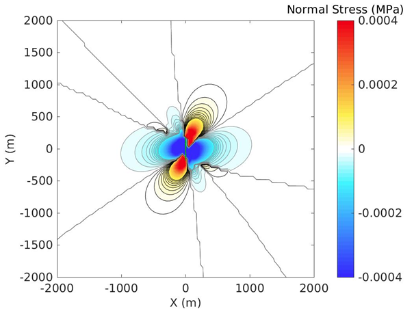
Figure 3. An example stress map at 50 m resolution

References

Freed, A. M., 2005. Earthquake triggering by static, dynamic, and postseismic stress. Annu Rev Earth Pl Sc, Volume 33, pp. 335-367.

Kilb, D., Gomberg, J. & Bodin, P., 2002. Aftershock triggering by complete Coulomb stress. J Geophys Res-Sol Ea, 107(B4), p. ESE 2–1 – ESE 2–14.

Okada, Y., 1992. Internal deformation due to shear and tensile faults in a half-space. B Seismol SocAm, 82(2), pp. 1018-1040.

Shapiro, S. A. et al., 2006. Fluid induced seismicity guided by a continental fault: Injection experiment of 2004/2005 at the German deep drilling site (KTB). Geophys Res Lett, 33(1), p. L01309.

Westwood, R. F., Toon, S. M. & Cassidy, N. J., under review. A sensitivity analysis of the effect of pumping parameters on hydraulic fracture networks and local stresses during Shale Gas operations. Fuel.