Page History
| Anchor | ||||
|---|---|---|---|---|
|
| Info |
|---|
To estimate ground motion prediction equation (GMPE). The GMPE relate relates ground motion parameters, usually amplitude parameters, to sets of independent variables representing the cause of the motion. The following independent variables could be taking taken into account: characteristic of the path, source and site. Moreover, the non-linearity of ground vibration propagation on short distances from the epicenter is supported by using 'h' as the common/fix depth factor h is estimated so that the standard error of estimation is the leastminimised. The finale model final model is estimated using ordinary one-stage regression method in three steps, includes including the statistical and physical correctness consistency of the model, estimation of the fixed depth (if its it's chosen as a parameter) and residuals analysis. |
REFERENCES Document Repository
CATEGORY Probabilistic Seismic Hazard Analysis
KEYWORDS Ground motion
CITATION Please acknowledge use of this application in your work:
IS-EPOS. (2019). Ground Motion Prediction Equations [Web applications]. Retrieved from https://tcs.ah-epos.eu/
Information
The complex model is

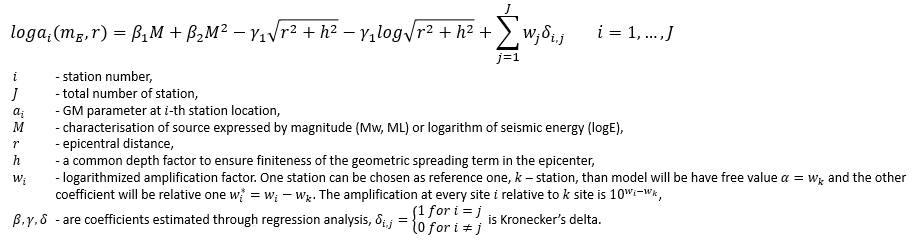
The model takes into account successively the successive increase of GM parameter along with the increase of source size, non-linear source influence, non-elastic damping, non-linear geometric scattering, and influence of site effect at the station. The model can be customized by choosing customised by selecting any parts.
The Ordinary ordinary one-stage regression method is used.
This application is prepared in 3 steps and the model can be improved in two of them model can be improved.
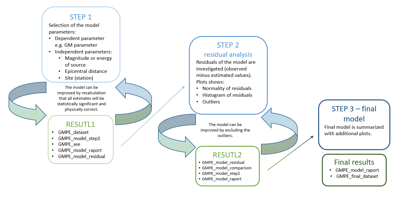
Step by Step
- Preparation of the data - GM parameters Parameters Catalog is needed.
To prepare GM parameters Catalog as tParameters Catalog 2 files are needed: the 1st input file is a a Seismic Catalog and the 2nd input file is Ground Motion Catalog from the same Episode (AH EPISODES). Thus, choose a catalog Catalog and GM Catalog from a selected episode. Then run Ground Motion Parameters Catalog builder,and as a result will be GM parameters Catalog. result GM Parameters Catalog will be created.
The part of the GM parameters Parameters Catalog can be used with Catalog filter. It is worth to remove smal values of PGA ef weak ground motion eg. PGA <=0.03 m/s2. - Selection of the model parameters (STEP 1 of analysis)
After the User adds the Application into his/her personal workspace, the following window appear on the screen (Figure 1), and the user is now requested to fill the fields shown on in Figure 1:
GM Parameters: The user may choose from all available ground motion parameters which were available in GM Catalog.
Source characteristic parameter: The user may choose from all available source parameter which parameters which were available in Catalog. The model may contain M, M2, both or none of them. Recommended is to choose select both and check their statistical significance in results. When coefficients or one of them is insignificant, they can be remove removed from the model.
Path characteristic: The model may contain R, logR, both or none of them. Additionally, epicentral distance may be calculated with fixed depth ('h' parameter in the model). 'h' parameter can be estimated (then option Estimate depth with model should be chosen)or can be type typed (the value is given in kilometerkilometres). Recommended is to choose select estimation of fix depth with model and choose both coefficients and check their statistical significance in results. When coefficients or one of them is insignificant, they can be remove removed from the model.
Site characteristic: Site characteristic depends on station position.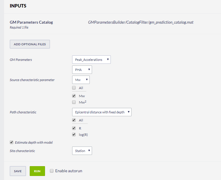
Figure 1. Input window of Ground Motion Prediction Equations: GMPE calculation After defining the aforementioned parameters mentioned above, the user shall click on the
 button (Figure 1), and the calculations are performed. The output is soon to will be created soon.
The output results include:
gmpe_model_report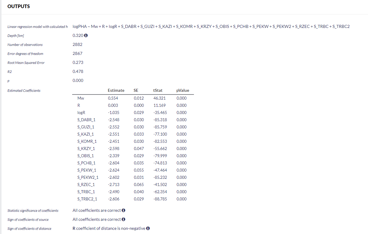
Figure 2. Ground Motion Prediction Equations model report.
R2 - (R-squared value) - coefficient of determination is the proportion of the variance in the dependent variable that is predictable from the independent variable(s). It shows in the percentage of which the model explains the variability in the response.
Root Mean Square Error (RMSE) - is a frequently used measure of the differences between values (sample or population values) predicted by a model or an estimator and the values observed.
p - probability o F-statistic for testing statistical significance of the model.
SEE chart (when 'h' is chosen as one of coefficient)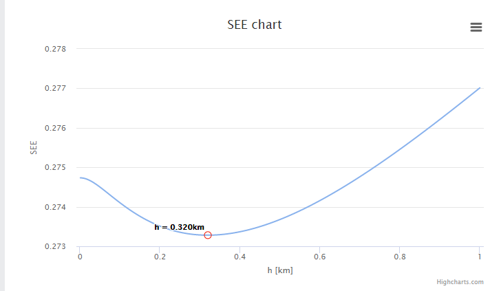
Figure 3. SEE plot.
Additional results:
gmpe_dataset.mat - especial prepared Matlab table mat file with chosen parameters based on GM Parameters Catalog with chosen parameters for which GMPE is calculeted.calculated,
gmpe_model_residuals - especial prepared Matlab table .mat - mat file with residuals of the model,
gmpe_model_step1.mat - mat file with results of 1. step.- Improving the model:
According to the result - especially the mainly statistical significance of coefficients and its physical correctness its physical consistency - the model can be improveimproved. To improve the model choose , click on the .
.
In this case R coefficient case, the 'R' coefficient of distance will be remove because removed because it is non-negative.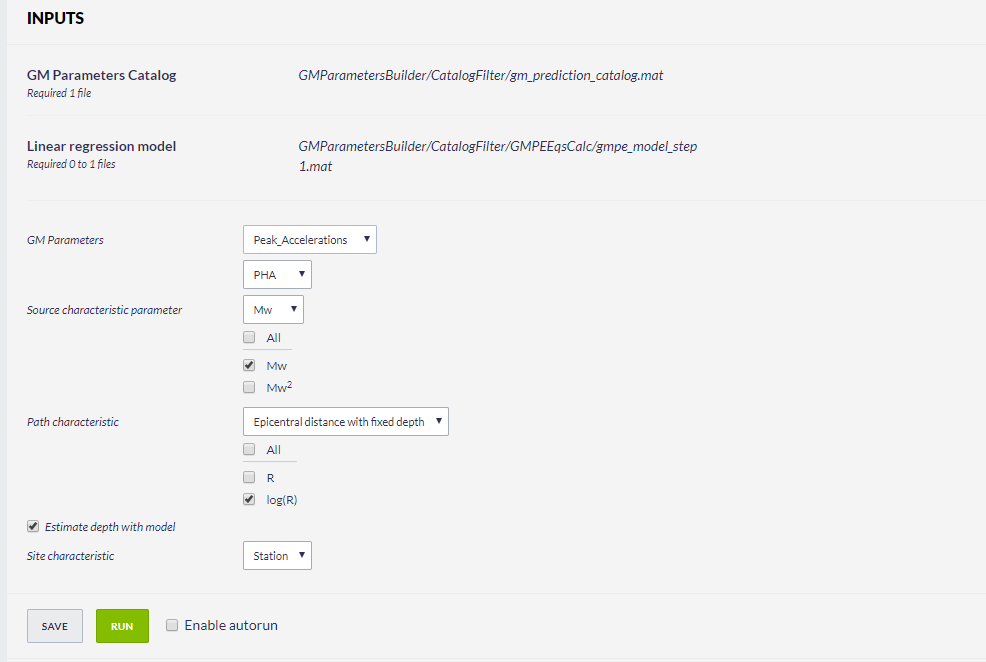
the
Figure 4. Input window of GMPE recalculation.
The result: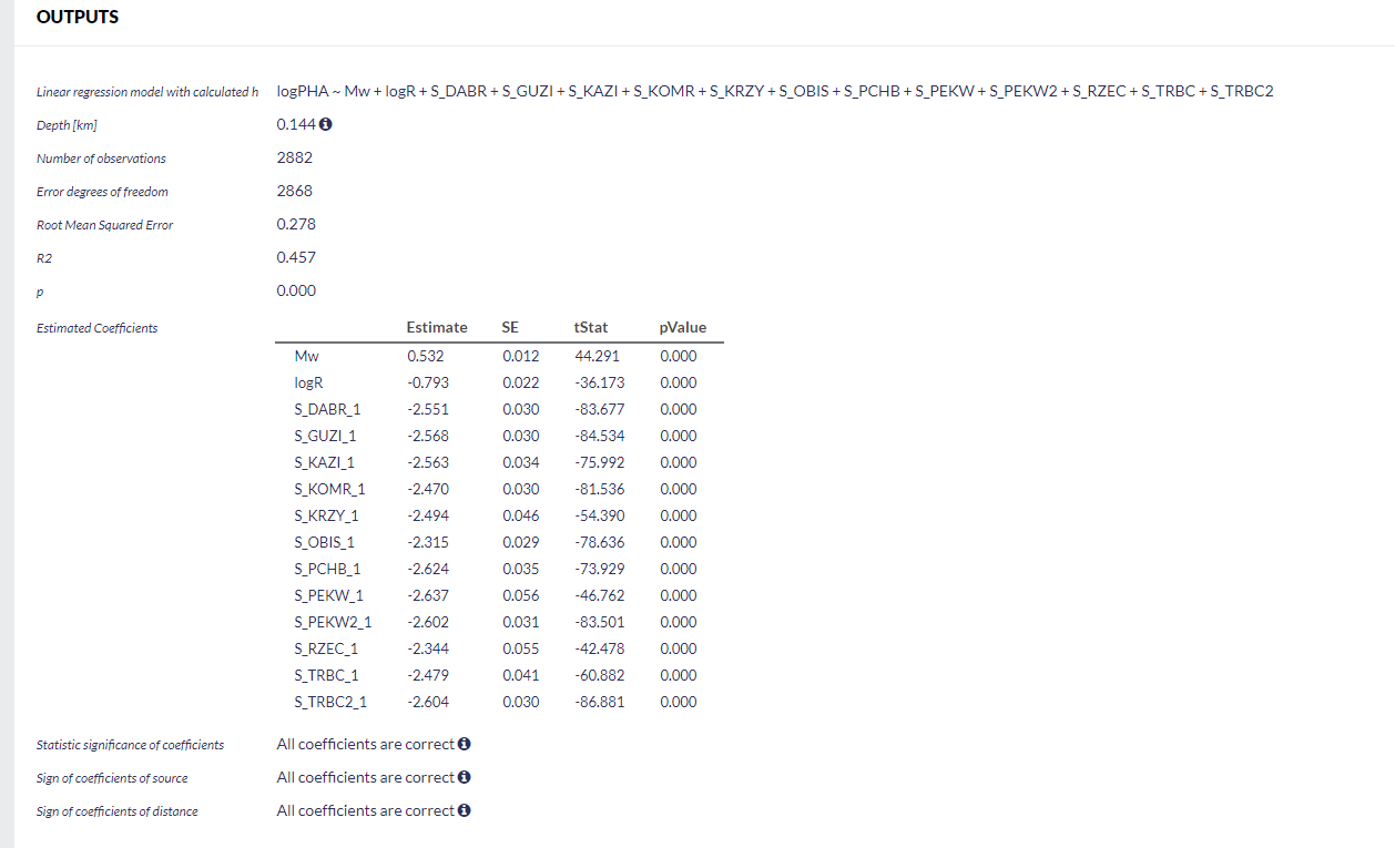
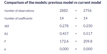
As a additionally Figure 5. Result of recalculated model. - As an additional result, after the improving the model, the comparison of previous vs current model parameter appearappears.
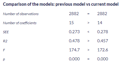
The The new (recalculated) model is better when SEE is 'SEE' and 'p' are smaller, R2 is bigger, F is bigger and p is smaller and 'R2' and 'F' are bigger than in the previous model.
This model does not need improving. All coefficient are proper and statistically significant. Recalculation The calculation can be done so many time until as many times until the results are satisfactory.
- Residual Analysis:
After receiving the satisfying model, the residual analysis can be perform performed (STEP2 of analysis). To start choose .
.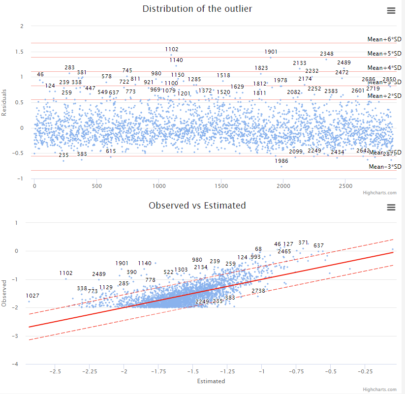
Figure 6. Residuals plots.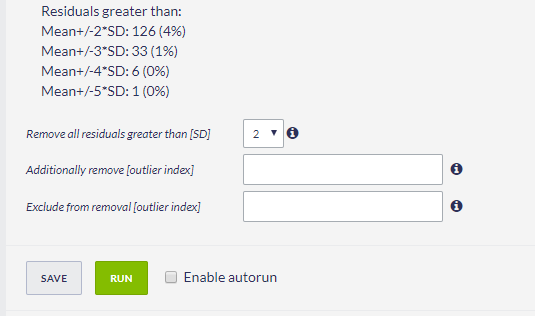
Figure 7. Input window of remove residuals part.
The results: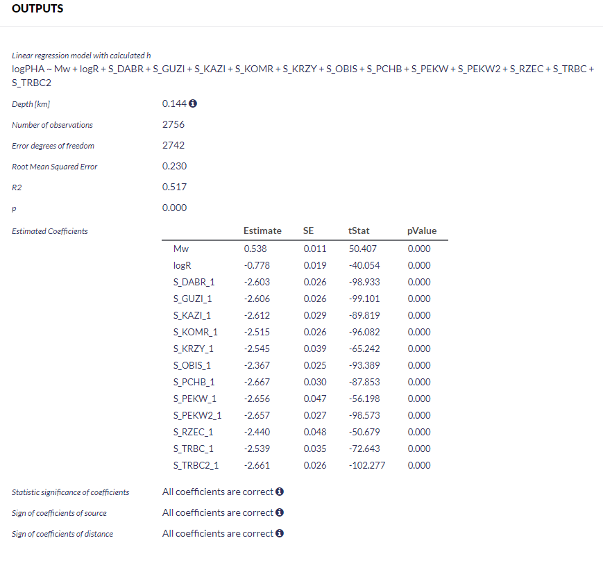
According to Figure 8. Results of the model after the removing outlieres.
Depending on the result - especially spreading of outliers when scattering of residuals is evident - the analysis can be repeated. To repeat choose choose the result will be. Recalculation Recalculation can be done so many time done as many times until the results are satisfactory. - Summary:
After receiving the satisfying model, the residual analysis final model can be perform performed (STEP3 of analysis). To calculate the final last model with additional plot plots, please select .
.
The final output results include:
gmpe_model_raport, gmpe_model_dataset, figures (Normal probability plot of residuals, box plot - residuals according to the station, Mw vs residuals, r vs residuals).
There is also possibility to a possibility to configure selected figures based n on used and estimated parametersestimated parameters.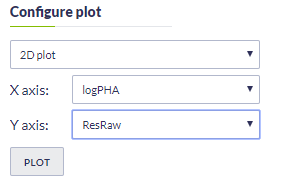

Overview
Content Tools