InSilicoLab for Chemistry
InSilicoLab is a collection of tools intended to assist the researcher in performing complex experiments of computational chemistry. It facilitates preparation of input files and submitting the jobs to the grid infrastructure, controls job execution, collects the output files and performs basic analysis of results. The user-defined experiment can be stored to allow for easy repetition of computational procedure. InSilicoLab integrates with the grid storage providing access to the user data.
Currently, experiments available in InSilicoLab for Chemistry are:
- Trajectory Sculptor
- Quantum-chemical calculations experiment
- Cubegen experiment
The InSilicoLab portal can be accessed at https://insilicolab.chemia.plgrid.pl.
Note: It is advisable to start reading with the basic user's manual before advancing to this one.
Getting access to InSilicoLab
InSilicoLab is accessible to anyone registered as a PL-Grid user or having a valid Grid Certificate and belonging to vo.plgrid.pl or gaussian Virtual Organisations. PL-Grid users may log in using their PL-Grid credentials by choosing to log in with OpenID or with personal certificate. In case of OpenID login, the user will be redirected to the OpenID page, where they will be prompted for PL-Grid login and password or a Grid Certificate associated with the account. If certificate login is chosen, the InSilicoLab portal will read the certificate installed in the user's browser. Note: If the certificate is not present or the user declines to use it for authentication, browser restart would be required to log in with the certificate again.
More information about activating and accessing the service for PL-Grid users can be found here.
InSilicoLab offers also anonymous preview access. It includes manipulation of molecular dynamics trajectories with use of Trajectory Sculptor and viewing sample experiments and their data. Downloading any data is not possible in the anonymous mode.
Trajectory Sculptor
Sequential MD/QC approach is often used in explicit solvent modeling. In the first step, Molecular Dynamics simulations (classical or ab initio) are employed to generate atomistic structures of the system and their evolution in time. In the next step, quantum-chemical calculations are performed for selected part of the system (solute molecule and closest solvent molecules in its solvation shell) to calculate required properties (such as potential energy, excitation energies, chemical shifts, etc.). Such calculations are usually repeated for series of frames chosen from the trajectory.
Trajectory Sculptor is a tool facilitating data preparation in such a procedure. It assists the user in trajectory analysis, selection of the part of studied system and extraction of solute-solvent geometries from selected frames. Data can then be passed to another InSilicoLab experiment to set-up and execute quantum-chemical calculations, monitor their status, collect output files and perform basic post-processing of the results.
Trajectory Sculptor can work with trajectories obtained from many MD packages. With support for multiple types of solvent molecules and flexible construction of the solvation shell (choice of distance metric and selection of solvent molecules) this tool is applicable to a wide range of systems, including solvent mixtures, electrolyte solutions or ionic liquids.
All steps of MD trajectory analysis in Trajectory Sculptor are described in detail in following sections.
Accessing Trajectory Sculptor
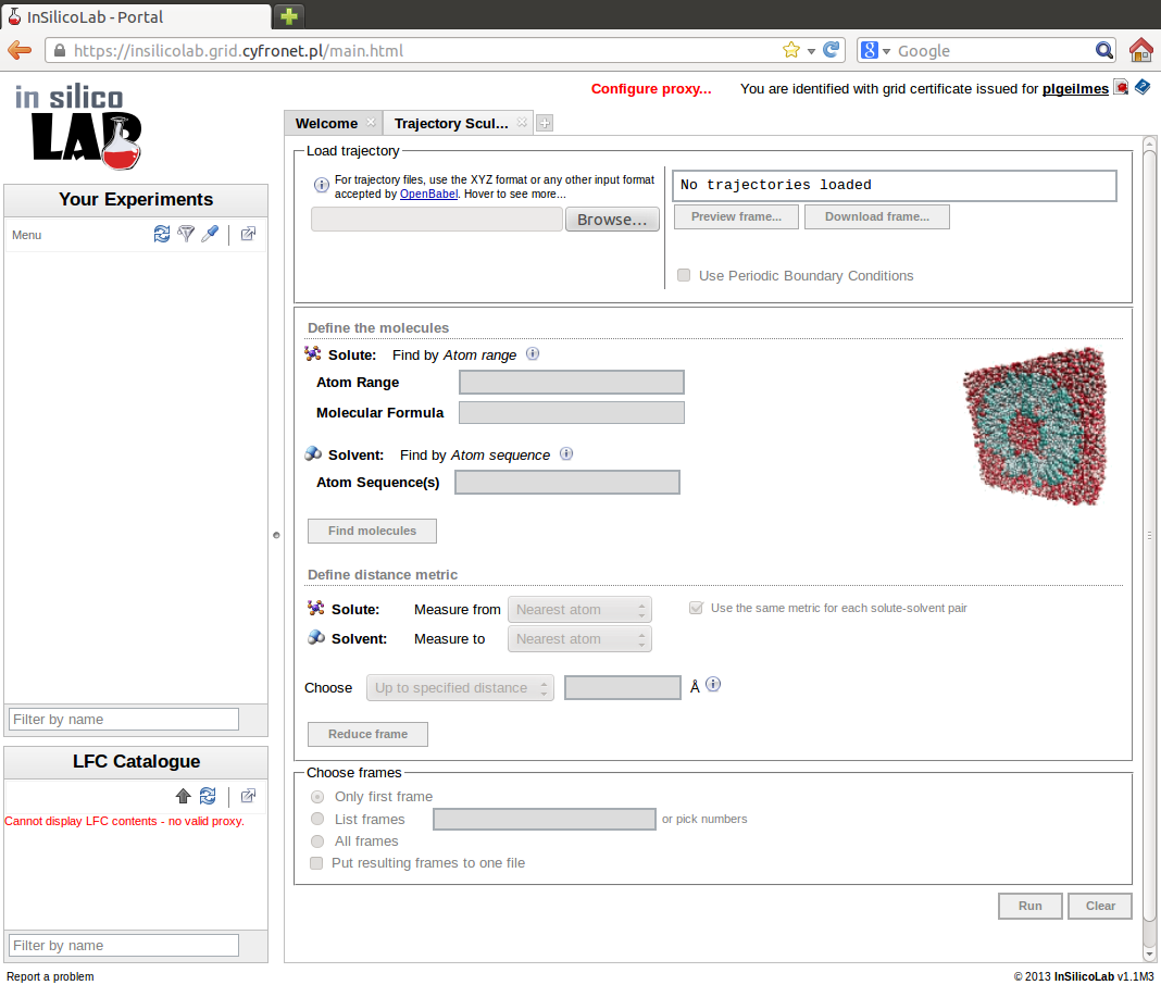
Trajectory Sculptor can be accessed from the main page after entering the portal. After choosing Trajectory Sculptor from the list of new experiments to create, the Trajectory Sculptor interface, similar to the one in the picture is shown.
Trajectory upload
Basic format of the MD trajectory files used by Trajectory Sculptor is the xyz format. However, trajectory may be supplied in other format recognized by OpenBabel in which case it will be automatically converted to xyz file.
Note: trajectory files generated by some popular MD programs including NAMD, Gromacs, AMBER or Tinker can be saved as xyz files using VMD software.
In order to make the analysis of the trajectory file possible in Trajectory Sculptor, several requirements have to be fulfilled:
- correct chemical symbols must be used in the trajectory file (i.e. no nonstandard labels)
- currently only one solute molecule is allowed
- sequence of atoms must be the same in all frames
- identity of molecules must be preserved in the course of MD run (no changes in bonding pattern)
- if periodic boundary conditions are used, all periods must be kept constant; only rectangular boxes are supported
To upload the trajectory file, press the Browse... button in the Load trajectory panel and select the file. After the file has been successfully loaded, a message appears in the message box on the right of the panel and the number of frames found in the file is displayed:
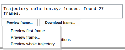
Uploaded trajectory may be previewed in the Jmol viewer using the Preview frame... button and selecting one of available options
- Preview first frame
- Preview frame... (on choosing this option a message box appears allowing to enter desired frame number)
- Preview whole trajectory
Note: In case the trajectory has only one frame or it is in format other than xyz and exceeds the size limit, only the Preview whole trajectory option is available. The size limit is introduced due to performance issues of OpenBabel which is used to extract the chosen frame. The limits are: 10,000 atoms or 100 frames or 200,000 atoms*frames. In case of xyz files these limits do not apply as a more optimal processing is chosen. Still, if the trajectory has only one frame, all the options are equal to Preview whole trajectory.
Selected frames may be also downloaded back in the xyz format using the Download frame... button and providing frame number (the same size limits as for frame preview apply here).
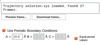
If periodic boundary conditions (PBC) were used in the MD simulation, period lengths must be provided. To do this check the Use Periodic Boundary Conditions checkbox, then enter period values (in Å) for three perpendicular directions. If the simulation box was a cube, select Equal period values checkbox in which case only one value (for period A) is necessary, the other two are automatically duplicated.
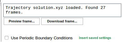
PBC information for the system is stored within the Trajectory Sculptor. If the user downloads the same file in the future, PBC settings can be easily recalled using the Insert saved settings option.
System specification
The next step of MD trajectory analysis is the specification of molecules (solute and solvent) present in the system. Specification is entered in the Define the molecules panel.
Solute molecule is defined by the range of atom numbers within the frame entered in the Atom Range field in Solute section. Sequence of atom numbers must be continuous and is given as hyphen-separated two integers. Optionally, sequence of atom labels for the solute may be entered in the Molecular Formula field. This input is used only for verification.
Solvent molecules are defined by the sequence of chemical symbols entered in the Atom sequence(s) field in the Solvent section. The sequence of symbols must match exactly sequence of atoms in the solvent molecule in the trajectory, e.g. OHH defines water molecule. All molecules of given type in the trajectory must have the same order of atom labels. If more than one type of solvent is present in the system, another Atom sequence(s) field may be created by clicking the Add... command. Sequence of symbols for the next solvent may be then entered. Note: solvents should be defined in the order of first appearance in the trajectory file.
On clicking the Find molecules button the first frame of the trajectory is analyzed and the information about molecules found in the system is displayed:
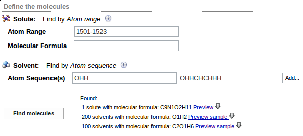
In the above example one solute molecule consisting of 23 atoms with the formula C9NO2H11, 200 water molecules (defined as OHH sequence) and 100 ethanol molecules (defined as OHHCHCHHH) are found in the frame. Solute molecule and example of solvent molecules may be viewed on choosing Preview or Preview sample option, respectively. Their geometries may be downloaded in the xyz format on pressing the arrow symbol.
Distance metric definition
To select solvent molecules closest to the solute one must define how the distance between two molecules is defined. Trajectory Sculptor allows several ways of measuring solute-solvent distances.
To define the distance metric for solute-solvent pair two reference points are defined: one anchored at the solute molecule, the other at the solvent. Distance is then defined as the distance measured from one reference point to the other. Reference points are selected from the Solute: Measure from and the Solvent: Measure to lists.
Four possible reference points may be defined:
- Chosen atom - reference point is selected atom of the molecule; its number has to be entered in the atom number field. Atom numbers are counted within the molecule, not in the whole system, i.e. atom no. 2 means the second atom in the molecule, although it may be the atom number 1502 in the frame
- Nearest atom - reference point is the atom of the molecule closest to the other reference point (at the other molecule)
- Geometric center
- Center of mass - reference point is calculated using the atomic masses of elements; isotopes are not taken into account
Any combination of these reference points is allowed.
Examples of distance metric definitions are:
- solute: nearest atom, solvent: nearest atom - distance is defined as the distance between closest atoms of the two molecules
- solute: chosen atom no. 10, solvent: nearest atom - distance is measured between atom no. 10 in the solute molecule and the closest to it atom from the solvent molecule
- solute: center of mass, solvent: chosen atom no. 2 - distance is measured between center of mass of the solute molecule and the second atom of the solvent
If more than one solvent type is present, different distance metric may be defined for each type of solute-solvent pair as in the following example:
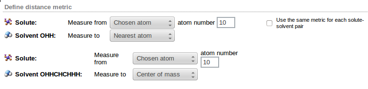
Checking the Use the same metric for each solute-solvent pair option facilitates entering the same definition for all solvents. Note, however, that this option is inactive if the Chosen atom reference point has been selected for the solute.
Selection of the solvation shell
After the solute-solvent distance metric has been defined it is possible to specify which solvent molecules should be included in the solvation shell. This is achieved by proper settings of the values in Choose option. Solvent molecules can be specified in two ways:
- Up to specified distance - all solvent molecules within the specified distance (in Å) are included in the solvation shell
- Closest molecules - given number of solvent molecules closest to the solute is selected
In both cases the solute-solvent distances are measured according to the distance metric defined for given solute-solvent pair.
If multiple types of solvent molecules are present, either one or many values may supplied for both options. If one value is given, it is used for all solvents. Alternatively, different values (separated by semicolons) may be specified for each type of the solvent; the numbers should be given in the same order as used in solvent specification.
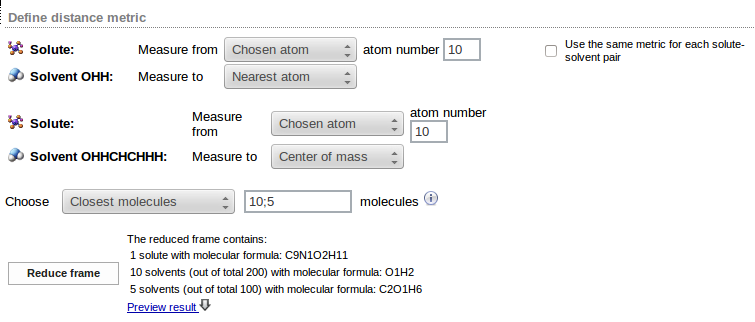
In the above example 10 water molecules and 5 ethanol molecules closest to the solute are selected. Solute-water distance is measured from the atom no. 10 in the solute molecule to the nearest atom of water molecule; solute-ethanol distance is measured from the atom no, 10 of solute to the center of mass of ethanol molecule.
The Reduce frame button may be used to analyze a sample frame (the first frame of the trajectory). Number of solvent molecules matching the requested criteria is displayed (in the example 11 water and 12 ethanol molecules were found within the 8Å distance from the solute):

and the sample of reduced frame may be previewed in Jmol using the Preview result link
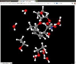
or downloaded as an xyz file on clicking on the arrow symbol.
Distance metric definition and the parameters of the Choose option may be changed as many times as necessary, therefore the Preview result command helps to find out the best distance metric and the appropriate way of selecting solvent molecules.
Final analysis of the trajectory
When the molecules in the system have been defined, the distance metric and the way of selecting molecules have been set up, the MD trajectory can be finally analyzed to extract solute with specified solvation shell from selected frames.
The Choose frames option allows to specify which frames should be analyzed:
- Only first frame
- List frames - allows to specify the list of frames
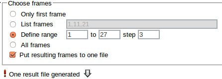
- Define range - allows to select numbers of the first and the last frame and the increment
- All frames
When the List frames has been used the frame numbers separated by commas can be entered
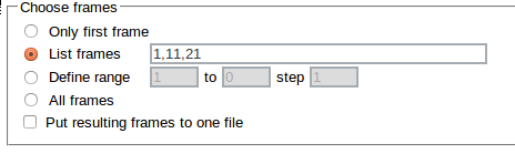
If more than one frame has been specified, the Put resulting frames to one file option can be checked to combine all reduced frames into one xyz file. If this option has been left unchecked, a separate xyz file is produced for each frame.
Clicking the Run button starts the analysis and reduction of the MD trajectory.
If the Put resulting frames to one file option has been used, the resulting xyz file may downloaded by clicking on the arrow.
Otherwise several files are created:
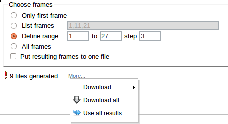
They can be downloaded individually (Download), downloaded as one xyz file (Download all) stored or passed to another InSilicoLab experiment (Use all results).
Quantum-chemical calculations experiment
This experiment facilitates preparation of input files for quantum-chemical calculations and execution of jobs on the PLGrid infrastructure.
Accessing the QC experiment
QC experiment can be accessed from the main page after entering the portal - by choosing Quantum Chemistry experiment from the list of new experiments to create.
Another possibility is to invoke the QC experiment from another InSilicoLab experiment (e.g. Trajectory Sculptor). In such case geometries of the system may be passed between experiments and they are immediately available as input data in the QC experiment interface.
Setting-up the QC experiment
The QC experiment is identified by the name entered in the field Short name. Optionally, more detailed description may be provided in the Description field. If no Short name is supplied, the contents of the Title section will be used. If both fields are empty, the "(no title)" will be used as a short name.
The geometry of the system may be entered from a file loaded in the Molecule Specification section. The type of the file may be specified in the opening window.
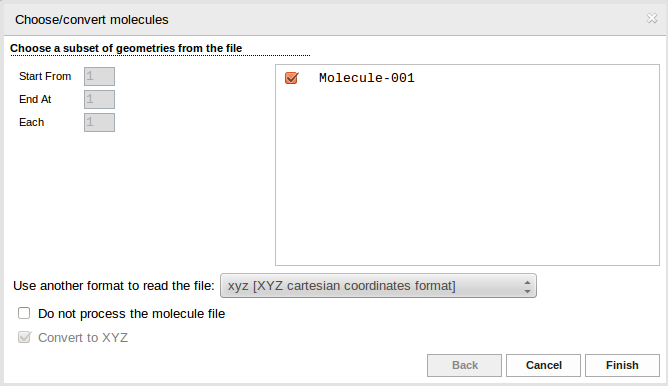
The system and the requested calculations are specified in the Input Data Specification section.
As a default, the file type is determined from the filename extension. Click Finish button to finish the specification of the geometry. If the QC calculations were invoked from another InSilicoLab experiment, the list of molecular geometries already contains the data passed from the other experiment.
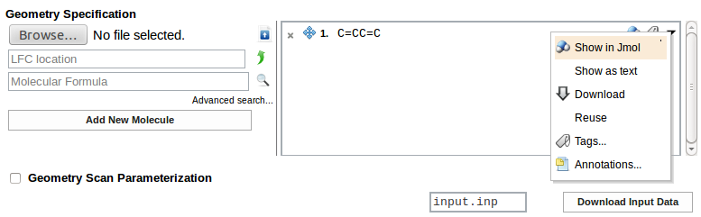
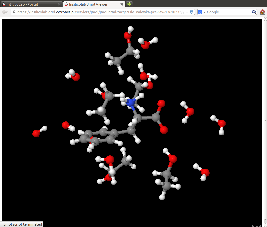
Structure of the system selected from the list may be visualized as an Jmol applet (Show in Jmol):
The software used in calculations can be selected from the list. Currently, three QC programs are supported:
- Gaussian 09
- GAMESS
- Turbomole
- Niedoida (QC package developed at the Faculty of Chemistry of the Jagiellonian University)
The fields needed to properly describe the calculations depend on the software chosen.
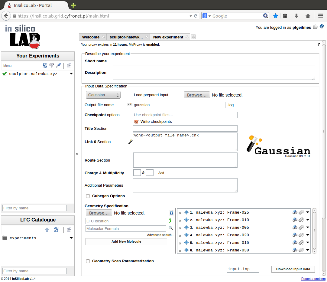
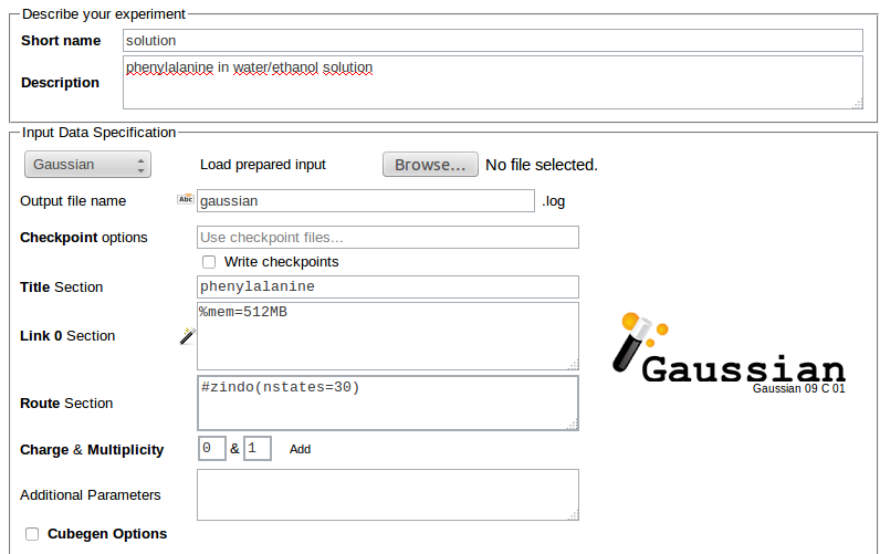
In the case of Gaussian 09 the following can be supplied:
- Title section - short description of the job (optional)
- Link 0 section - parameters of program execution such as memory and disk limits and the use of checkpoint files (optional)
- Route section - QC method and type of calculations (required)
- Charge & Multiplicity of the system (required)
- Additional parameters - added to the Gaussian input file after the geometry specification (optional)
- Cubegen options - to generate a Gaussian cube file (optional)
- Geometry Scan Parameterization - allow performing geometry scan of the structure (optional)
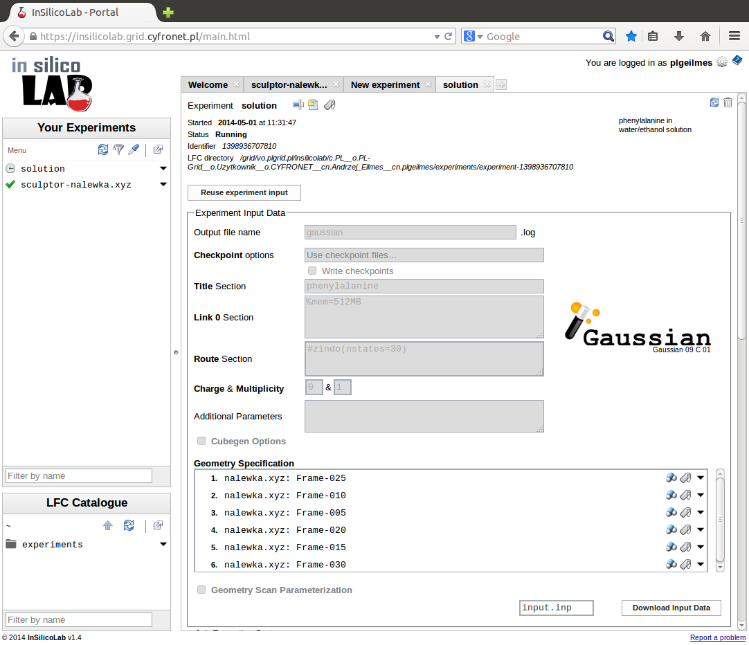
For example, the input for Gaussian ZINDO calculations of 30 lowest electronic excitations for a phenylalanine molecule in a solution using structures prepared in Trajectory Sculptor and requesting 512MB RAM for each job may read:
Job execution
Clicking the Run button creates the input files based on the supplied geometries and parameters entered in the Input Data Specification. The jobs are then submitted for execution to the PLGrid.
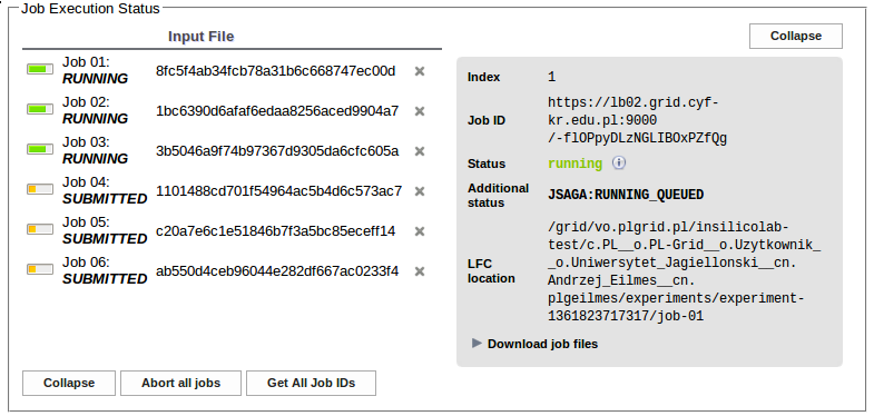
In the Job Execution Status section one may trace the progress of calculations. The job status changes from EXTERNAL through SUBMITTED and RUNNING to FINISHED.
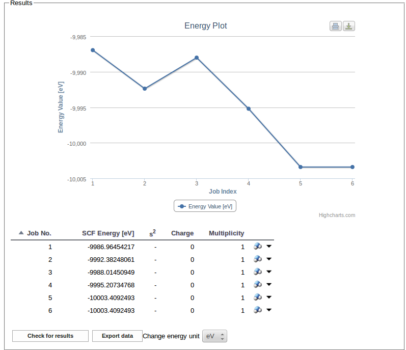
Results of finished jobs are used to update the table and the plot of SCF energy values:
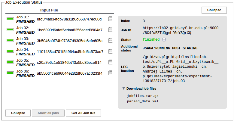
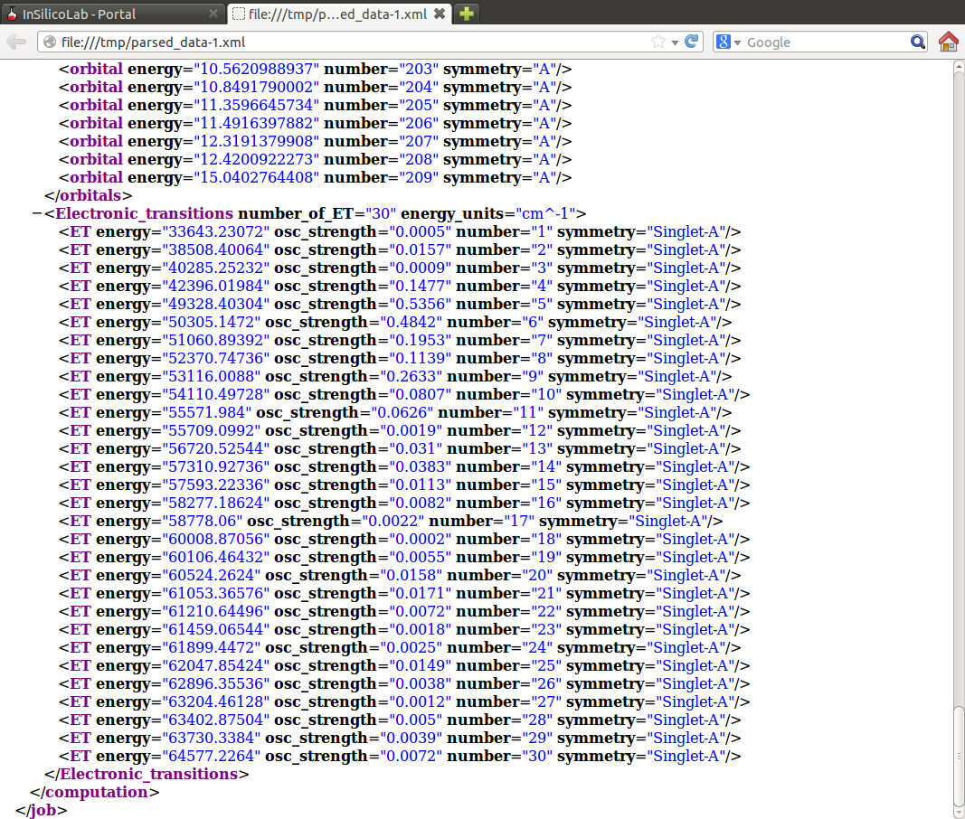
For each job the Download job files list may be used to select and download the files associated with the job: input, checkpoint and output files as a single .tar.gz file or the XML file containing the results extracted from the output.
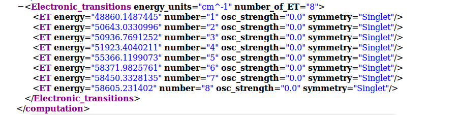
In the above example of ZINDO calculations such file contains the list of calculated transition energies and oscillator strengths.
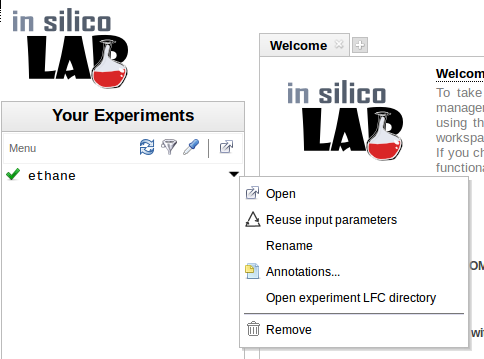
User can store the parameters of the experiment and job files for future retrieval or easy repetition of calculations:
Using niedoida program in general quantum-chemistry experiment
Niedoida is a quantum-chemical package developed at the Faculty of Chemistry of the Jagiellonian University in collaboration with the Academic Computer Centre ACK Cyfronet AGH.
Program implements standard methods of quantum-chemistry
- Hartree-Fock
- Density Functional Theory and TDDFT
- post-HF methods: MP2 and CIS
MP2 calculations can be accelerated by the resolution-of-identity technique (RI-MP2; efficient for large basis sets) or Laplace-Transform MP2 (effective for spatially extended systems).
Program features implementation of "dressed"-TD DFT incorporating corrections from doubly-excited states.
LT-MP2 calculations example
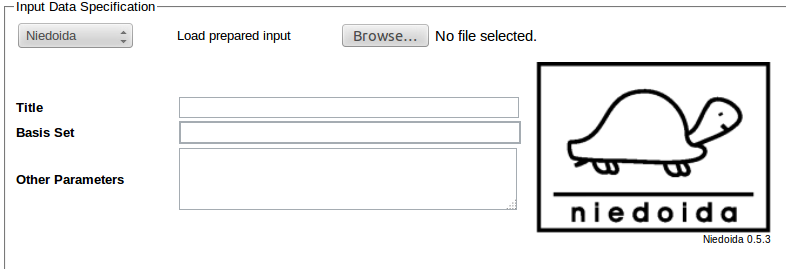
To use the program its name needs to be selected from the list of programs in the Input Data Specification section:
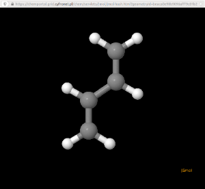
Coordinates of the system can be entered in the Geometry Specification section. Uploaded geometry can be viewed as Jmol applet on clicking the molecule icon next to the file name. Butadiene molecule is used in the example.
Required input data should be entered in the Input Data Specification section:
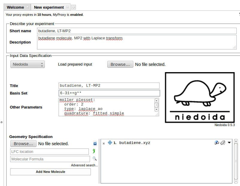
In the above example 6-31++G** basis is requested for calculations (Basis Set field), other data are entered in Other Parameters field:
units: length: angstrom energy: hartreemoller_plesset: order: 2 type: laplace_ao quadrature: fitted_simple
Here we have specified units of distance (default unit is bohr) and energy. MP2 calculations with Laplace-Transform have been requested.
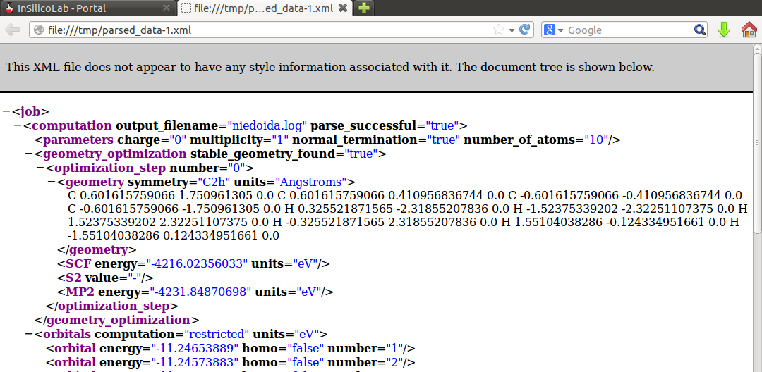
Calculations are initiated on clicking the Run button. After successful completion output file (niedoida.log) and parsed XML data can be downloaded.
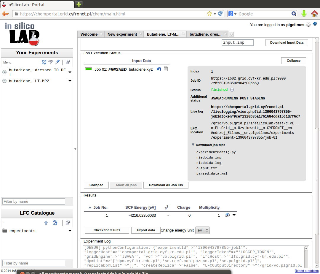
Note that in the Results window the HF SCF energy is displayed, therefore to read the MP2 energy log file needs to be inspected or (more conveniently) the requested value can be found in the parsed_data.xml file:
dressed-TD DFT calculations example
Selection of the program and entering the coordinates of butadiene molecule can be done as in the former example.
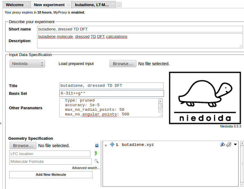
Necessary data to be entered as Input Data Specification are the Basis Set (here 6-311++G**) and Other Parameters:
units: length: angstrom energy: hartreetheory: pbe0td: type: tda multiplicity: 1 no_states: 8 no_roots: 16 no_iterations: 100 diagonalization_threshold: 0.00001 max_no_dressing_iterations: 100 dress_delta_energy: 0.3 max_no_davidson_dressing_iterations: 30 dress_davidson_threshold: 0.0001 dress_state: 5integration_params: cache_size: 64grid: type: pruned accuracy: 1e-5 max_no_radial_points: 50 max_no_angular_points: 500
PBE0 functional has been chosen for TD DFT calculations employing Tamm-Dancoff approximation. Eight excited states have been requested. Corrections from double excitations should be calculated for the 5th state using energy window of 0.3 hatree.
The XML file available after job completion contains the uncorrected TDA results:
To access the results of the "dressed" calculations output file (niedoida.log) needs to be checked.
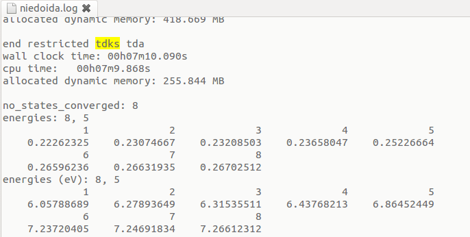
Results of the uncorrected TDA calculations are displayed after the "end restricted tdks tda" line:
Corrected energies are available after the last "end restricted tdks dressed tda" statement:
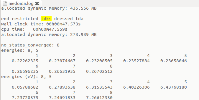
In the above example corrections arising from double excited states lowered the energy of the 5th state from 6.865 to 6.438 eV.
Cubegen
This experiment is used to generate Gaussian cube files.
Optional description of the experiment consists of its Short name and the Description used to annotate the experiment.
To generate the cube file it is necessary to provide (in the section Checkpoint Specification) a checkpoint file containing the data saved from a previous Gaussian run. The file can be downloaded by the user (Add file location list) or retrieved from a LFC storage (LFC location - open the browser and allows the user to select the file). The file stored in LFC directory can be generated in an earlier general QC experiment (option requesting saving checkpoint files had to be used).
Input Data Specification describes the type and parameters of the cube file:
- Cube filename
- Cube type - on clicking the wand icon a list of possible choices is presented, e.g. electron density, molecular orbital, spin density, potential, gradient, etc.; for detailed description of cube types the User is referred to the Gaussian cubegen manual
- Include header option (yes or no)
- Cube specification - controls the size/density and units of the cube grid, as described in the cubegen manual
The experiment is started on clicking Run button.
Overview
Content Tools